Starting with dBASE PLUS 8 with ADO, the new SQL Builder feature is one that dBase believes will offer years of expanded capability and functionality.  One of the main reasons for replacing the older SQL Designer is that we needed to be able to add additional databases quickly and easily.  The new SQL Builder supports the latest databases, in a fast, consistent interface, with additional room for enhancement and upgrades.

The new SQL Builder also gives much more control over the type and style of the SQL being generated and saved.  The SQL Builder allows developers to create very simple, to very deep and difficult, SQL right from the drag-and-drop interface, which will be covered later in this documentation.

Keep in mind, to work with SQL Builder, you need basic knowledge of SQL concepts.  SQL Builder will help you to write correct SQL code while hiding the technical details, but only by understanding the SQL principles will it be possible to achieve the desired results.

Selecting a database access method (ADO or BDE)

The first step in using the new SQL Builder is picking the data-access method to be used, either ADO or BDE.  Note:  At this time, SQL Builder does not support mixing different data-access methods from within an SQL statement.

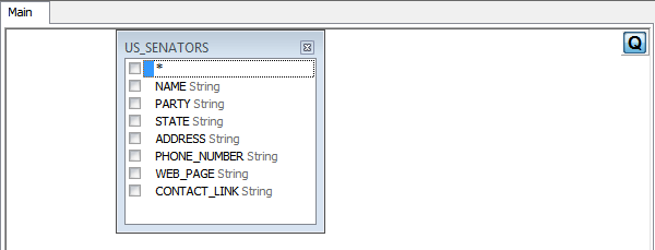
The first thing to do is pick the SQL tab on the Navigator or click the File|New|SQL from the menu system.  Below is an example of the Navigator being used to create a new SQL statement using the SQL Builder:

Using the Navigator to start a new SQL statement

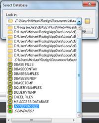
Once the Navigator is on the SQL tab, you can select the [New SQL] in the top left corner of the Navigator.  Double-click and you will be offered a database connection dialog will appear:

List of all the databases or aliases to connect

In the above example notice that there are two different listings; one states  STANDARD1 and the other is MYTESTMYSQL.  Each of these two items represent a different data-access layer.  The STANDARD1 is using the BDE to make connections while the MYTESTMYSQL is connecting to a remote-cloud server running MySQL.

Therefore, if the developer selelcts the STANDARD1, then the BDE will be used for database access.  If on the other hand, the developer chooses MYTESTMYSQL then ADO will be used.  Note:  While ADO is being used, the MYSQL database is actually using the ODBC driver socket that is part of the ADO technology.

     
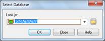
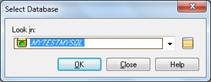
Connecting to the BDE                                          Connecting to ADO

Once you choose the data-access technology, press the OK button to continue and the rest of the SQL Builder interface will be loaded with the tables associated with the selection of the data-access technology.

2-Way SQL Development

The first thing you should notice when starting up SQL Builder is that it fits the dBASE development paradigm rather well.  It supports the concept of 2-Way development.  If you don’t remember what 2-Way development is, it is the process if you make changes on the GUI designer, the code will automatically reflect those changes, and if you make changes to the code, the GUI designer will automatically show those changes in real-time.

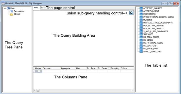
SQL Builder interface

The main window of SQL Builder can be divided into the following parts:

·         The Query Building Area is the main area where the visual representation of the query will be displayed.  This area allows you to define source database objects and derived tables, define links between them, and configure the properties of tables and links.

·         The Columns Pane is located below the query building area.  It is used to perform all the necessary operations with query output columns and expressions.  Here, you can define the field aliases, sorting and grouping, and define criteria.

·         The Table list is located at the right.  Here, you can see and browse your table’s objects.

·         The Query Tree Pane is located at the left.  Here, you can browse your query and quickly locate any part of it.

·         The page control above the query building area will allow you to switch between the main query and sub-queries.

·         The small area in the corner of the query building area with the "Q" letter is the union sub-query handling control.  Here, you can add new union sub-queries and perform all the necessary operations with them using the popup menu.

                  
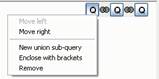
Union Sub-Query operations                 Operations with brackets                       Select union joining operator

Again, at any time, the developer can see the SQL code behind the GUI based SQL Builder by simply pressing the F12 key to toggle between graphic view and code view.  This can be done at any time during the development process.  Again, remember that any changes to the GUI will change the code and any code changes will show in the GUI representation.  This will be highlighted below:

        
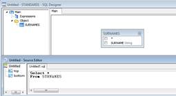
This is a SQL base code                                                        Clicked the Surnames, notice the code difference

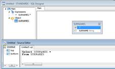
Now change the code back to the “Select * from SURNAMES” and look at the difference in the GUI, as shown below:

         
Remove the SURNAMES.* from the code                             Notice the check in the GUI is missing from the * in SURNAMES table

Finally, we should highlight the menu that is associated with the SQL Builder.

SQL Builder’s menu

Starting from the left:

·         New – this gives you a dropdown to pick or create a “new” something

·         Open – this will open and load a file

·         Save – this will save a file

·         Print – this will print the active file

·         Cut – this is the cut for the selected editor for the clipboard

·         Copy – this is the copy for the selected editor for the clipboard

·         Paste – this is the paste for the selected editor for the clipboard

·         Execute – run and display the results of the SQL statement

·         Design – this will return the product to the Design surface, the Execute and Design can toggle

·         Add Table – this will add a table or allow for another database alias to be picked, this can also be done with the hotkey {CTRL-A}

·         Context Sensitive Help – this will take you to the help associated with the particular in focus part.  For example, if you are on the Select statement, then press Help will start on the Select statement outline

Drag and Drop execution

SQL Builder allows for full drag-and-drop functionality.  Use the mouse to select a Table from the Table list on the right side of the interface and hold down the left-mouse and drag the table onto the Query Building area as shown below:

SQL Builder drag procedure in progress

Once you have the table in the desired location, release the left-mouse key and the table will be placed in that exact spot.

The tables in the Query Builder area can be moved by using the same drag-and-drop technique used to put tables on the Query Builder area.  While the query relationships will be covered later in the documentation, the drag-and-drop features area is also used to create relationships between tables as shown below:

Drag-and-Drop – relationships

In the Query Building area, there is another way to add Tables objects to the designer surface.  Right-mouse click on the Query Building area and the following dialog will be displayed:

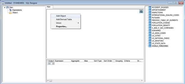
Right-mouse click on the Query Builder area and select ADD Object

Once selected, the Add Object should give the following dialog:

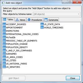
Ability to add additional Table objects (Tables, Views, Procedures, and Synonyms)

Select the desired object and click the Add Object button to add it to the Query Builder area.  You can select one or several objects by holding the Ctrl key and then press the Add Object button to add these objects to the query.  You can repeat this operation several times.  After you finish adding objects, press the Close button to hide this window.

Simple Query

SQL Builder can be used to create any kind of SQL, from the very basic to the very complex.  How complex?  SQL Builder allows you to build complex SQL queries with Unions, Sub Queries, and Derived Tables visually.  In this section, the steps needed to perform a simple query will be outlined.

To start, click on the Navigator and select the SQL Tab.  There you will see a [New SQL] item and double-click on that time.  This will display the Select Database dialog; pick a data connection that has tables or databases associated with it.  After clicking the OK button this will start the SQL Builder graphical user interface, as shown below:

Using the SQL Builder GUI to build a simple query

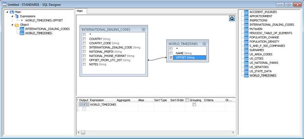
For this example, the database picked will be the US_SENATORS.  This is a small database and is very quick to show the results.  Click and drag a table from the Table List on the right and drop it in the Query Builder area in the top-center.  Notice the table is represented by a box with all of the defined columns displayed as below:

Table in the Query Builder area

The first thing that needs to occur in the example is choosing which fields you want to display.  This is a Simple click procedure in SQL Builder.  If you want all of the fields to show in a particular Table, you can just click the top-level “*” as shown below:

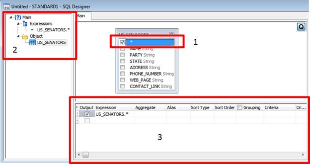
Selecting fields to be part of the SQL statement

There are 3 main areas that should be looked at in the above image.  The first area is the table.  Notice that it has the checkmark beside the “*” field, which means all fields will be included in the SQL statement. 

The SQL code generated:  Select US_SENATORS.* From US_SENATORS

The next area is the Query pane on the left that outlines the SQL being generated.  Finally, review the contents of the Columns pane (number 3), where it also highlights which fields have been selected.

If you only need a few of the fields, instead of selecting the “*” field, you can click the desired field and a checkmark will be display beside that particular field, as shown below:

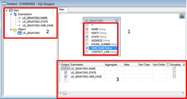
SQL Builder showing selected developer-defined fields

In the #1 pane, the selected fields have a checkmark beside them, the #2 pane shows each field in the SQL statement, and the #3 pane is showing the items ready for advanced SQL features.  These field selections can be changed at any time during the development process or later when loaded back into the system.

Once the simple SQL has been defined, the next steps in going through the SQL development process is to Save the SQL statement.  For a more in-depth review of the Save procedure, please refer to the “Saving an SQL statement” later in the SQL Builder documentation.  The fastest way to save is to click the Save icon on the toolbar, which will display the Save dialog.  Name the SQL and hit the OK button, as shown below:

Save SQL dialog

The dialog will disappear and the SQL will now be named and will show in the interface:

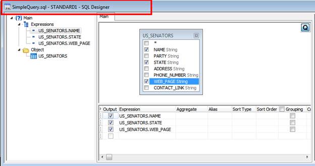
Named SQL query

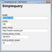
Once the SQL has been saved, it can now be executed by clicking the Execute toolbar button.  For a more in-depth review of the Execute procedure, please refer to the “Executing an SQL statement” section later in the SQL Builder documentation.  A new window with the results of the SQL statement will be generated:

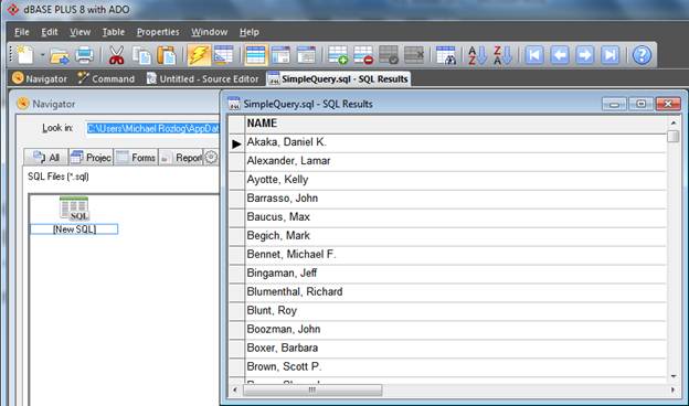
Notice the generated results for the SQL statement

Please note that when executing an SQL statement, the SQL Builder will disappear.  In addition, when the Results window is clicked, the associated toolbar will be changed as well.  When in the Results view, you have the ability to change or modify the contents of the data being displayed.

If you are fine with the results, or notice additional changes need to be made, you can simply click the Design toolbar button and the SQL Builder GUI will reappear and the Results window will be closed automatically.

Those are the steps for creating a simple query using the SQL Builder found inside dBASE PLUS 8 with ADO.

Executing an SQL statement

In dBASE PLUS 8 with ADO, the Execute and Design toolbar buttons in the Execution toolbar are closely tied together:

Execute and Design toolbar buttons

Any time after the SQL has been saved, you will have the option to “Execute” the SQL statement.  By clicking on the Lightning Bolt button.  The “Execute” process can also be activated using the View|SQL Results menu item on the main product menu, or alternatively it can be activated with the F2 keyboard shortcut.

Once the results have been reviewed, you can return to the SQL Builder design surface by clicking on the “Design” toolbar button to the right of the “Execute” toolbar button.  This will close the results window and return you back the SQL design surface.  This operation can also be activated using the View|SQL Design menu item on the main menu.

You can go-back-and-forth between Execute and Design. 

During the “Execute” phase, when the Results window has focus or is clicked on, the toolbar will be updated to include various additional functionality as listed below:

SQL Results toolbar

Starting from the left:

·         New – this gives you a dropdown to pick or create a “new” something

·         Open – this will open and load a file

·         Save – this will save a file

·         Print – this will print the active file

·         Cut – this is the cut for the selected editor for the clipboard

·         Copy – this is the copy for the selected editor for the clipboard

·         Paste – this is the paste for the selected editor for the clipboard

·         Execute – run and display the results of the SQL statement

·         Design – this will return the product to the Design surface, the Execute and Design can toggle

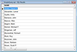
·         Grid layout – this is the default layout for the SQL Results:

·         Columnar layout – this will change the results to a columnar layout:

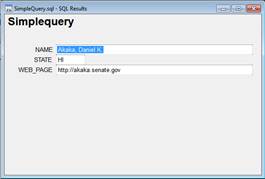
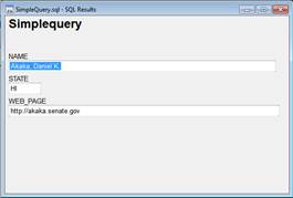
·         Form layout – this will put the SQL results into a form layout:

·         Add Row – this will add a row at the bottom of the result set, and can be executed using the keyboard shortcut {CTRL-A}

·         Delete Row – this will delete the active row in the result set

·         Save Row – this will save or post the updates back to the underlying database through the respective data-access (ADO or BDE) and it can also be executed using the keyboard shortcut {CTRL-S}

·         Abandon Row – this will abandon any changes made

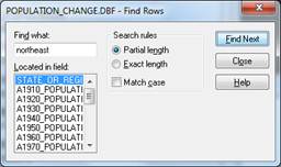
·         Find Rows – This will return a set of rows and can be implemented using the keyboard shortcut {CTRL-F}

·         Sort Ascending – this will put the results in a sort order from a – z

·         Sort Descending – this will put the results in a sort order from z – a

·         First Row – This will move the cursor to the first record in the result set.  It can also be activated by using the keyboard shortcut {CTRL-HOME}

·         Previous Row – This will move the cursor to the prior record in the result set

·         Next Row – This will move the cursor to the next record in the result set

·         Last Row – This will move the cursor to the last record in the result set.  It can also be activated by using the keyboard shortcut {CTRL-END}

·         Context Sensitive Help – this will take you to the help associated with the particular in focus part.  For example, if you are on the Select statement, the the Help will start on the Select statement outline

The “Execute” process gives you full control over the look and presentation of the data, plus it allows you the ability to manipulate the dataset at time of execution.

Saving an SQL statement

In SQL Builder, before any SQL statements can be “Executed” they must be Saved.  This can be accomplished by clicking the Save toolbar button or by click the File|Save or File|Save As… main menu, menu items.  This will display the standard save dialog as shown below:

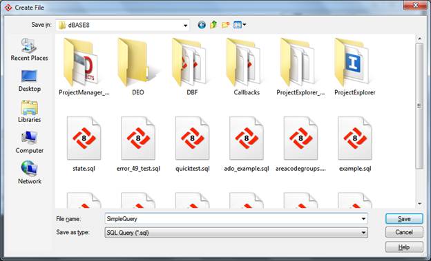
Save dialog – Create a file

Once the file has been named and pointed to the proper location, you can click the Save button to finish the save operation.

Loading an existing SQL statement

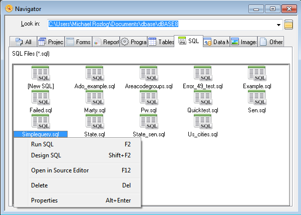
SQL Builder can be activated by loading a file with SQL inside that has a file extension of .sql, or by finding the specific SQL file in the Navigator as shown below:

Loading an SQL file using the Navigator to active SQL Builder

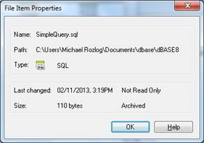
Using the Navigator gives the most options when loading an SQL file.  Right-mouse clicks on the particular SQL file to be presented with the above options.  You can Run SQL {F2} key, or open the SQL Builder designer using the Design SQL {Shift+F2} key, or go right to the source F12 key, or Delete {Del} Key the SQL file.  Finally, they could get the SQL File properties {Alt+Enter}, as shown below:

SQL file properties

It will show the name and location of the file.  When finished with the review, press the OK button to continue.

Joining Tables

SQL Builder fully supports Joins, and it automatically understands how to create Inner Joins with little fuss.  The join type that is created by default is INNER JOIN, which is fine in most cases.  However, for those servers that have no support of a JOIN clause, SQL Builder adds this condition to the WHERE part of the query, which is the case for dBASE (.dbf and .db) files.  There are some additional rules that must be followed when it comes to JOINs in dBASE:

·         All joins are left-to-right outer joins.

·         All join are equi-joins.

·         All join conditions are satisfied by indexes.

·         Output ordering is not defined.

·         The query contains no elements listed above that would prevent single-table updatability.

Conversely, for a little more information on Joins, here is an excellent explanation of Inner / Outer Joins types:

Assuming you're joining on columns with no duplicates, which is by far the most common case:

·         An inner join of A and B gives the result of A intersect B, i.e. the inner part of a venn diagram intersection.

·         An outer join of A and B gives the results of A union B, i.e. the outer parts of a venn diagram union.

Examples

Suppose you have two Tables, with a single column each, and data as follows:

Note that (1,2) are unique to A, (3,4) are common, and (5,6) are unique to B.

Inner join
An inner join using either of the equivalent queries gives the intersection of the two tables, i.e. the two rows they have in common.

·         select* from a INNER JOIN b on a.a = b.b;

·         select a.*,b.*  from a,b where a.a = b.b;

Left outer join

A left outer join will give all rows in A, plus any common rows in B.

·         select * from a LEFT OUTER JOIN b on a.a = b.b;

·         select a.*,b.*  from a,b where a.a = b.b(+);

Full outer join

A full outer join will give you the union of A and B, i.e. All the rows in A and all the rows in B. If something in A doesn't have a corresponding datum in B, then the B portion is null, and vice versa.

·         select * from a FULL OUTER JOIN b on a.a = b.b;

Taken from an excellent post and response from Mark Harrison from StackOverflow.com here:  http://stackoverflow.com/questions/38549/difference-between-inner-and-outer-join  (Above format modified for docs)

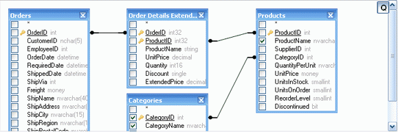
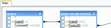
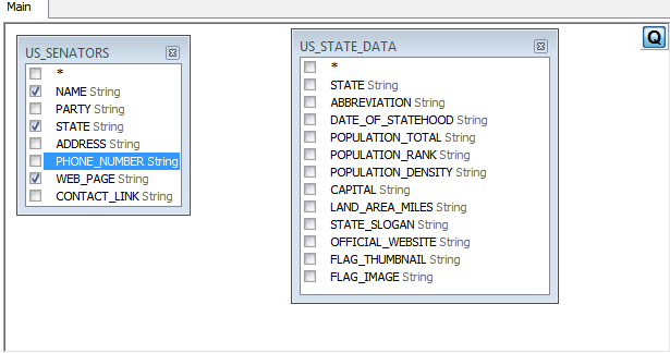
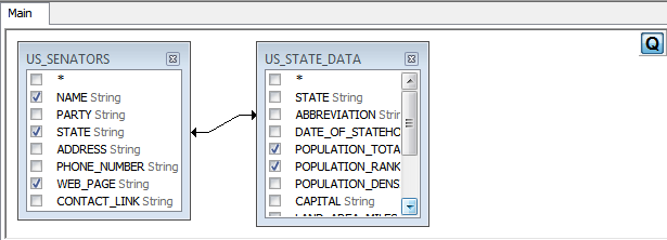
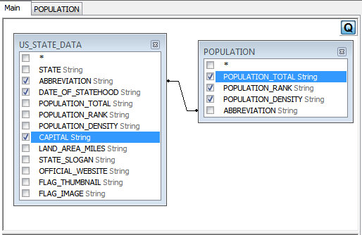
Our example will include two tables that have related information.  Table A (US_SENATORS) and Table B (US_STATE_DATA) are listed below for reference:

Two reference tables used for a simple JOIN

For this example, the Result set should include:

·         US_SENATORS – Name

·         US_SENATORS – State

·         US_SENATORS – Web_Page

·         US_STATE_DATA – Population_Total

·         US_STATE_DATA – Population_Rank

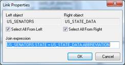
Before the JOIN can be created, SQL Builder needs to have included fields marked.  This means that Population_total and Population_rank need to be checkmarked.  The US_SENATORS – State field is a 2 character abbreviation.  That means the linkage between the two tables will be using that field and the US_STATE_DATA – Abbreviation field.

To create a link between two objects (i.e. join them) manually, you select the field you want to link and drag it to the corresponding field of the other object.  After you finish dragging, a line connecting the linked fields will appear.  Key cardinality symbols are placed at the ends of link when the corresponding relationship exists in the database.  The results are shown below:

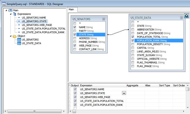
Showing a JOIN between two tables

In the above screen shot, notice that in the Query Tree pane (Left) that the US_SENATORS.STATE is selected and the same field in the Columns Pane (bottom) is selected, along with the drop-down arrow on the field as well.  This is a quick way to go from field to field.

The code that was generated for this particular SQL looks like the following:

Select US_SENATORS.NAME,  US_SENATORS.STATE,   US_SENATORS.WEB_PAGE,
           US_STATE_DATA.POPULATION_TOTAL,    
           US_STATE_DATA.POPULATION_RANK
From US_SENATORS
          Inner Join US_STATE_DATA On US_SENATORS.STATE =
                                                                      US_STATE_DATA.ABBREVIATION

When the Query is run, the Form view of the query looks like the following:

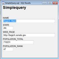
Form view of SQL statement using an INNER JOIN

To define join the type and other link properties, you can right click the link and select the Properties item from the context popup menu or double-click it to open the Link Properties dialog. 

Adding (Direction) to JOIN

Notice in the above dialog, that the direction is now going Left on the JOIN and the SQL generated will be reflected below:

Select US_SENATORS.NAME,  US_SENATORS.STATE,  US_SENATORS.WEB_PAGE,
           US_STATE_DATA.POPULATION_TOTAL,
           US_STATE_DATA.POPULATION_RANK
from US_SENATORS
         Left Join US_STATE_DATA On US_SENATORS.STATE =
                                                                  US_STATE_DATA.ABBREVIATION

In this simple example, the output looks the exact same as doing a simple INNER JOIN. 

There are times when you want to do a FULL JOIN and this is accomplished by making the linkage between the tables look like:

Doing a FULL JOIN on the two tables

The above source code would look like the following:

Select US_SENATORS.NAME, US_SENATORS.STATE, US_SENATORS.WEB_PAGE,
           US_STATE_DATA.POPULATION_TOTAL,
           US_STATE_DATA.POPULATION_RANK
From US_SENATORS
          Full Join US_STATE_DATA On US_SENATORS.STATE =
                                                                   US_STATE_DATA.ABBREVIATION

This can also be accomplished by right-mouse clicking on the linkage and selecting the Properties menu item:

Notice that both the Left and Right are selected and that represents a FULL JOIN.  The outcome of this SQL is still the same as the Simple INNER JOIN that was first created, however the need to show the code generation difference was needed.

Sorting

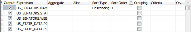
To define the sorting of the result dataset, you can use the Sort Type and Sort Order columns of the Columns Pane.  Using the same query that was used in the JOIN section of the documentation, set the SORT Type on the US_SENATOR – Name in a descending order as shown below:

Setting the Sort Type on a particular query

This will result in the following:

The Sort Order column allows you to setup the order in which the fields will be sorted, in case more than one field will be sorted.  To disable sorting, clear the Sort Type column for this field.  Now add Sort field and change the type and order, as shown below:

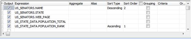
Setting Sort Type and Order for different results

Now the results are based on the Population.Rank, highest first, and then the SENATORS – Name, which result in the following:

             
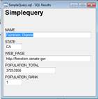
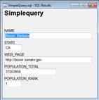
Initial result                                            Next record in line

Defining Criteria

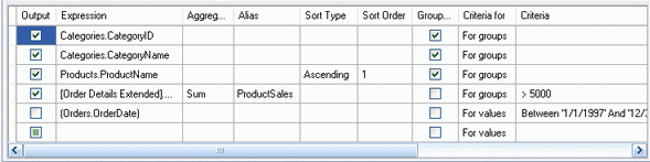
To define the criteria, you can use the Criteria and all of the Or columns of the Columns Pane (bottom).

In these cells, you should write the conditions omitting the expression itself.  For example, to get the following criteria in your query:

WHERE  (Field1 >= 10) AND (Field1 <= 20)

you should type ">= 10 AND <= 20" in Criteria cell of a Field1 expression.

Criteria placed in the Or columns will be grouped by columns using the AND operator and then concatenated in the WHERE (or HAVING) clause using the OR operator.  For example, this visual representation will produce the following SQL statement.  Please note that the criteria for Field1 are placed in both the Criteria and Or columns.

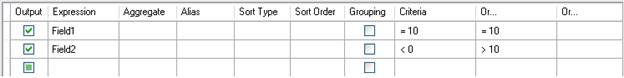
Showing criteria creation

WHERE (Field1= 10) AND ((Field2 < 0) OR (Field2 > 10))

Some expressions may be of the Boolean type, for example the EXISTS clause. In this case you should type "= True" in the Criteria column of such expressions or "= False" if you want to place a NOT operator before the expression.

Note: the most common practice to learn for how to build queries with criteria is to write it once by hand and see how it will be parsed and represented visually.

Grouping

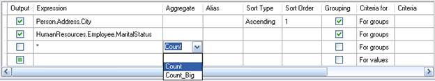
To build a query with grouping, you mark the expressions for grouping with the Grouping checkbox.

A query with grouping must have only grouping or aggregate expressions in the SELECT list.  Thus, SQL Builder allows you to set the Output checkbox for grouping and aggregate expressions.  If you try to set this checkbox for a column without the Grouping or Aggregate function set, a Grouping checkbox will be set automatically to maintain the validity of the result SQL query.

When the Columns Pane (bottom) contains columns marked with the Grouping checkbox, a new column called "Criteria for" appears in the grid.  This column specifies the appliance of criteria to the expression groups or to their values.

For example, you have a column "Quantity" with the Aggregate function "Avg" in your query and you type the "> 10" in the Criteria column.  Having the "for groups" value set in the Criteria for column, the result query will contain only groups with an average quantity greater than 10, and your query will have the "Avg(Quantity) > 10" condition in the HAVING clause.  Having the "for values" value set in the "Criteria for" column, the result query will calculate the Average aggregate function only for records with a Quantity value greater than 10, and your query will have the "Quantity > 10" condition in the WHERE clause.

Query Properties

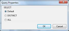
Various database server specific options are managed within the Query Properties dialog.  You can open it using the context popup menu of the Query Building Area.

Derived Tables

A Derived tble is a sub-query used as a datasource for the main query.

To add a derived table, you should right click the Query Building Area and select the Add Derived Table item from the context popup menu.

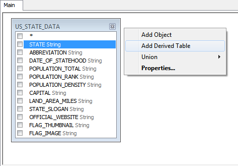
Creating a Derived Table

A new object representing the newly created derived table will be added to the query building area, and the corresponding tab will be created for it.  This tab allows you to build it visually in the same way as the main query.  Another way to switch to the corresponding derived table tab is to right click the caption of an object representing the derived table and select the "Switch to derived table" item from the context popup menu.

You can set an alias for the derived table the same way as for an ordinary database object.

You can always go back to the main query and switch to any sub-query or derived table using tabs above the Query Building Area (middle) or using the Query Structure Tree (Left).

Using a derived table

Unions

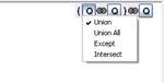
SQL Builder fully supports Unions.  UNION combines the results of two or more queries into a single result set that includes all the rows that belong to all queries in the union.

Union sub-queries are managed within the Union Panel in the top-right corner of the Query Building Area.  Initially there is only one union sub-query labeled with the "Q" letter.  All required operations are performed by means of context popup menus.

Union sub-queries can be grouped with other sub-queries and joined with different operators (UNION, UNION ALL, EXCEPT, INTERSECT).

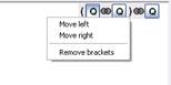
·         To add a new union sub-query, select the New Union sub-query menu item.

·         To enclose the sub-query in brackets, select the Enclose in Brackets menu item.

·         To move the sub-query or bracket to the top of the query (the topmost sub-query is the left one), select the Move Left menu item.

·         To move the sub-query or bracket to the bottom of the query, select the Move Right menu item.

·         To remove the sub-query or bracket, select the Remove menu item.

·         To change the union joining operator, select the necessary operator in the list of supported operators in the context popup menu.